Thermodynamic simulation-assisted random forest: Towards explainable fault diagnosis of combustion chamber components of marine diesel engines

Congcong Luoa, Minghang Zhaoa,*, Xuyun Fua, Shisheng Zhonga, Song Fub, Kai Zhangc, Xiaoxia Yud
aDepartment of Mechanical Engineering, Harbin Institute of Technology, Weihai 264209, China
bSchool of Mechatronics Engineering, Harbin Institute of Technology, Harbin 150001, China
cSchool of Mechanical Engineering, Southwest Jiaotong University, Chengdu 610031, China
dCollege of Mechanical Engineering, Chongqing University of Technology, Chongqing 400054, China

Abstract

Aiming at the challenges that traditional intelligent fault diagnosis methods of marine diesel engines often suffer low generalizability due to the lack of fault training samples, as well as poor explainability due to the insufficient incorporation of domain knowledge on fault mechanism, this paper develops a Thermodynamic Simulation-assisted Random Forest (TSRF).

The method reveals fault characteristics through thermodynamic simulations and incorporates them as prior knowledge when designing the intelligent fault diagnosis model. Firstly, five thermodynamic fault models are developed by fine-tuning the essential system parameters to correspond with the distinct attributes of different faults. Then, potential thermodynamic indicators of combustion chamber component degradation are identified through numerical simulation results.

By calculating SHapley Additive explanations (SHAP) values, a parameter selection process is conducted to retain only those variables demonstrating significant correlations with fault states. Finally, the selected parameters are leveraged to assess the condition of the combustion chamber. The proposed TSRF achieved exceptional classification performance, illustrating a mean accuracy of 99.07% on the fault dataset.

Keywords:
Marine Diesel Engine Fault Diagnosis Explainable AI SHAP

Motivation

In the fields of marine engineering and Prognostics and Health Management (PHM), the industry faces two persistent bottlenecks:

  • Data Scarcity: Marine diesel engines, especially the main engines on ocean-going vessels, are the heart of a ship. Any serious malfunction at sea risks a loss of propulsion, grounding, or even a major maritime disaster. For this reason, they are designed with extremely high safety margins, making the likelihood of a serious breakdown naturally low. In addition, the shipping industry follows strict preventive maintenance schedules, such as inspections based on running hours. Most parts prone to wear are replaced long before they actually fail or generate fault data. As a result, while we possess a vast amount of data on healthy engines and early wear patterns, there is a distinct lack of real-world data on total system failures.
  • The "Black Box" Problem: Since deep learning models typically lack transparency, engineers find it difficult to trust them without an explanation of the physical causality behind a fault. This opacity is particularly critical in the shipping industry, which is subject to rigorous oversight by classification societies. If an AI misdiagnosis precipitates a catastrophic failure like cylinder scuffing or a crankshaft fracture, and the system cannot identify whether the error stemmed from data bias, algorithmic flaws, or sensor drift, such untraceability is unacceptable in maritime accident investigations.

To address these challenges, we propose the TSRF method. This approach integrates physics-based mechanistic models with advanced explainability techniques. By leveraging high-fidelity simulation models to generate synthetic data, we effectively resolve the issue of data scarcity and ensure that diagnostic decisions adhere to fundamental thermodynamic principles.


Methodology

Our workflow consists of four distinct stages, as illustrated below:

  1. Thermodynamic Modeling: Rather than relying solely on physical test rigs, we constructed a high-fidelity 1-D thermodynamic model of a 6-cylinder marine diesel engine. The model was rigorously calibrated using real-world operational data, keeping simulation errors within 5%.
  2. Fault Injection: Based on the calibrated model, we adjusted the physical parameters to simulate five distinct combustion chamber faults, such as cylinder head cracks and piston ablation. We then generated a dataset that captures the full spectrum of fault severities observed in actual engines.
  3. Feature Selection via SHAP: We utilized SHAP values to quantitatively identify the critical features, including the 14 key parameters that drive the diagnostic decision.
  4. Classification: A Random Forest (RF) classifier was trained using this physics-enhanced dataset to achieve high diagnostic precision.
Structure of TSRF method combining Thermodynamic Simulation and Random Forest for Explainable AI

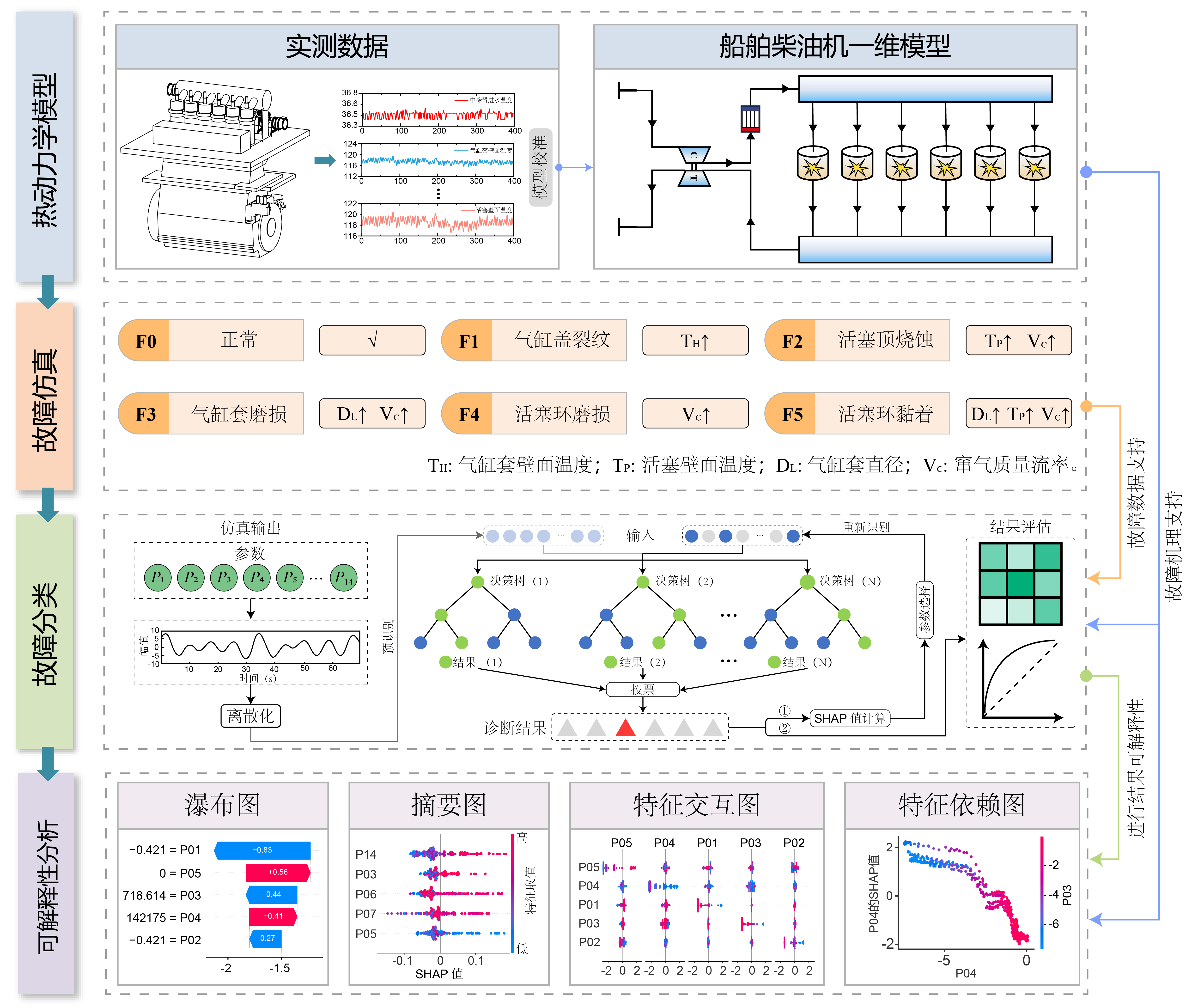
Figure 1: The structure of the proposed TSRF method.


Thermodynamic Modeling Details

To ensure high fidelity, we constructed a one-dimensional simulation model. This mechanism model balances physical accuracy with the computational efficiency required for dataset generation.

Model Topology

The engine is discretized into a network of flow pipes and functional components:

  • Core Power Unit: 6-cylinder, 2-stroke inline configuration.
  • Air Path System: Intake/Exhaust manifolds (PL1, PL2) connected via complex piping networks.
  • Boosting System: Turbocharger (TC1) coupled with an intercooler (CO1).

Calibration & Validation

Before fault injection, the baseline model was rigorously calibrated against empirical data.

  • Data Source: Real-world vessel data acquired via Data Collecting Module (DCM).
  • Validation: The deviation for critical parameters (e.g., Power, Exhaust Temp) was maintained within a ±5% error margin.
1-D thermodynamic simulation model

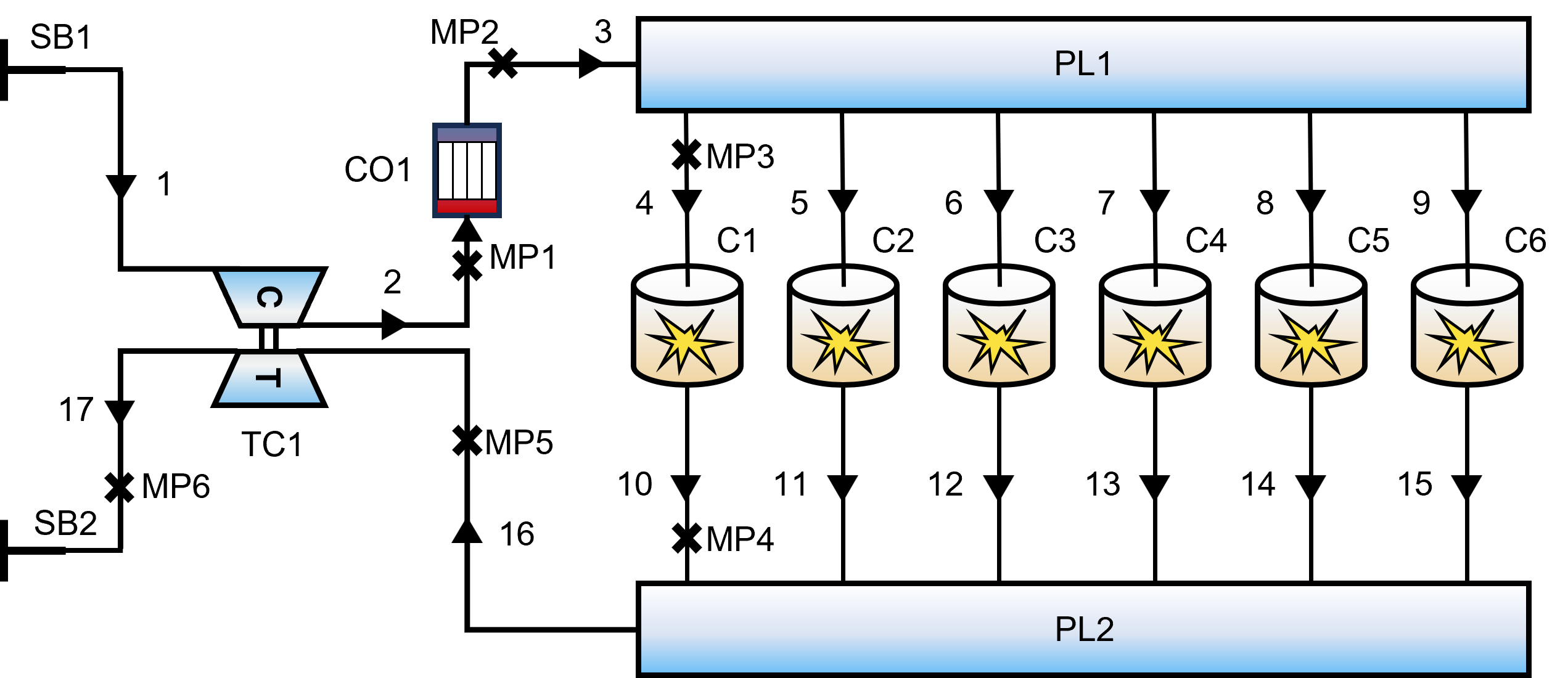
Figure 2: One-dimensional thermodynamic model of the diesel engine.

Model Validation Results

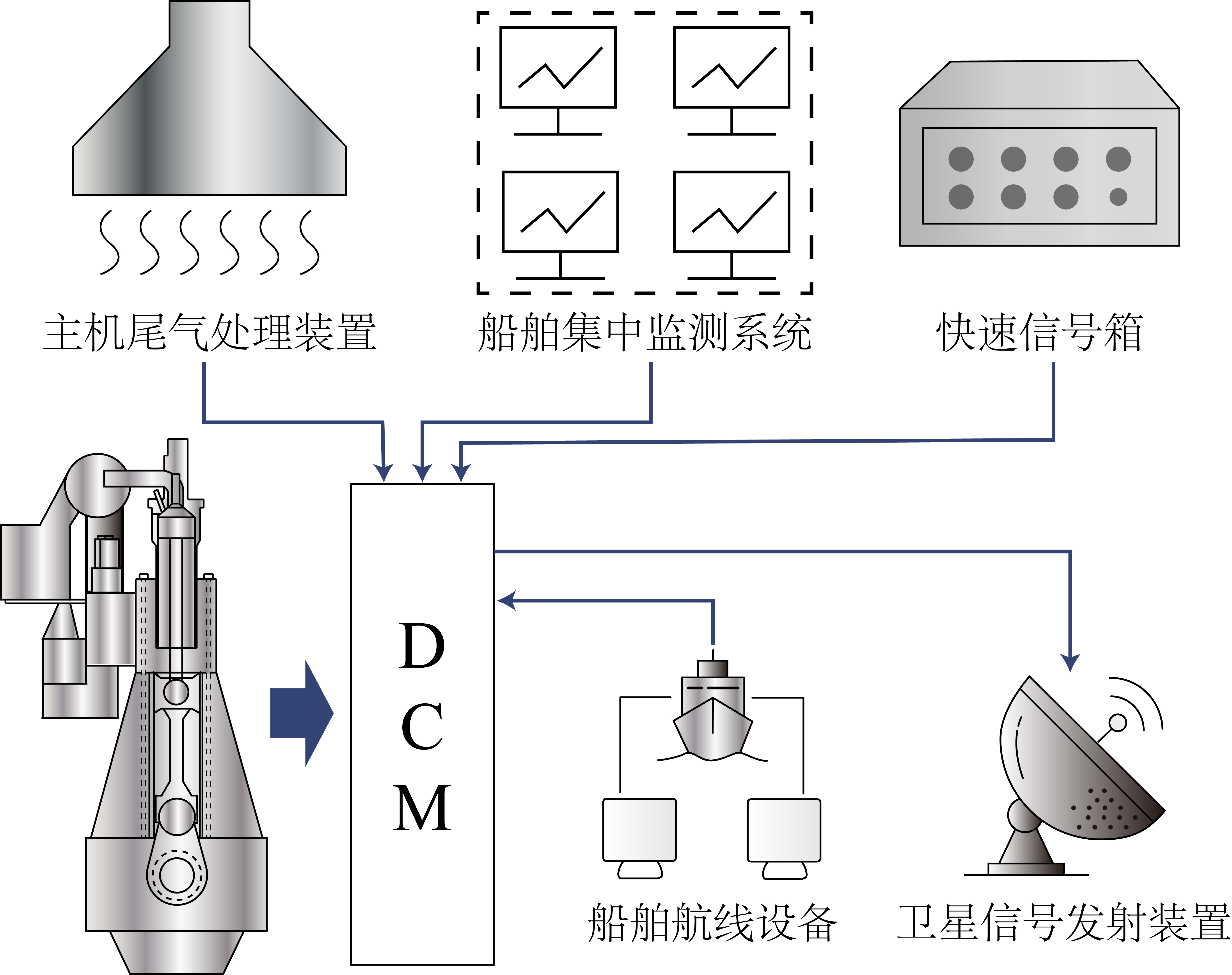
Figure 5: Data Collecting Module (DCM).

Fault Injection Mechanism

Since 1-D models cannot directly represent 3D structural defects, we employed a phenomenological mapping approach, translating physical degradation mechanisms into equivalent thermodynamic parameter shifts.

Fault Type Physical Mechanism Modeling Implementation
F1: Head Cracking Disrupted thermal conduction. Elevating Cylinder Head Surface Temp ($T_H$) to 346°C.
F2: Piston Ablation Material loss & seal compromise. Increasing Piston Temp ($T_P$) + minor blow-by (0.01 kg/s).
F3: Liner Wear Abrasive wear increases bore. Increasing Bore Diameter + substantial blow-by (0.03 kg/s).
F4: Ring Wear Gas leakage only. Modulation of Blow-by Mass Flow Rate (0.02 kg/s).
F5: Ring Sticking Friction & seal failure. Bore Dia. change + Elevated Liner Temp + Blow-by.

Explainability Analysis

A key innovation of our work is shifting the focus from "What is the fault?" to "Why is this the fault?". We demonstrate this capability through a case study on Piston Ring Wear (F4):

  • Local Interpretation (Waterfall Plot): The waterfall plot explains specific predictions. For instance, the model predicts "Ring Wear" because Blow-by Heat Flow (P06) and Blow-by Mass Flow (P07) exhibit specific values that increase the probability. This aligns with physics: ring wear compromises the seal, leading to gas leakage (blow-by).
  • Global Interpretation (Beeswarm Plot): Global analysis reveals the general rules learned by the model. We found that low values of Pre-turbo Exhaust Pressure (P11) are strong indicators of Ring Wear. Physically, this is consistent: worn rings allow gas to leak from the cylinder, reducing the energy available to the turbine.
SHAP Analysis,including Waterfall plot, beeswarm plot, interaction plot and dependence plot

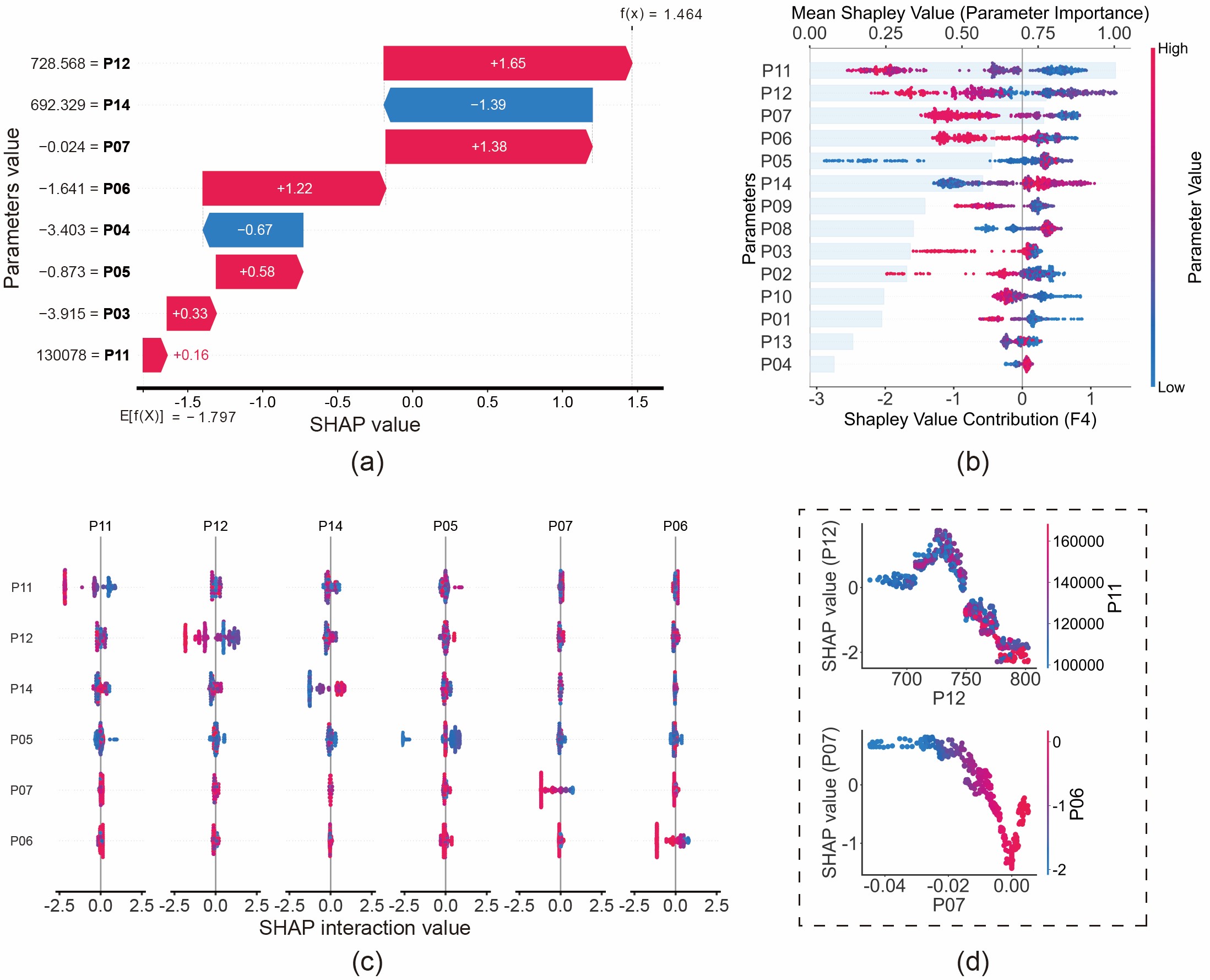
Figure 11: Fault analysis of piston ring wear (F4) based on SHAP values: (a) Waterfall plot; (b) Beeswarm plot; (c) Interaction plot; (d) Dependence plot.

Click to view SHAP Visualization Code (Python)

If you are interested in the implementation details of the figures above, here is the sample code used to generate the Waterfall, Beeswarm, Interaction, and Dependence plots.👇

import shap
import matplotlib.pyplot as plt
import numpy as np

# --- 0. Setup & Global Settings ---
plt.rcParams['font.family'] = 'Arial'
plt.rcParams['font.size'] = '24'
plt.rcParams['axes.unicode_minus'] = False

# Assumption: 'best_model' is your trained XGBoost/RF model
# Assumption: 'X_train' and 'X_test' are pandas DataFrames

# 1. Calculate SHAP values as Numpy Arrays (for Beeswarm, Dependence, Interaction)
explainer_tree = shap.TreeExplainer(best_model)
shap_values_numpy = explainer_tree.shap_values(X_train) 

# 2. Calculate SHAP values as Explanation Object (Specifically for Waterfall)
explainer_obj = shap.Explainer(best_model, X_test)
shap_values_obj = explainer_obj(X_test)


##################################################################
#                                                                #
#                      (a) Waterfall Plot                        #
#          Visualizes contribution for a single sample           #
#                                                                #
##################################################################

class_idx = 4  # Target class
sample_idx = 3 # Specific sample to explain

plt.figure()
shap.plots.waterfall(
    shap_values_obj[sample_idx, :, class_idx], 
    max_display=9, 
    show=False
)

# Customizing style
ax = plt.gca()
ax.set_xlabel(ax.get_xlabel(), fontsize=36)
ax.set_ylabel(ax.get_ylabel(), fontsize=36)
ax.spines['bottom'].set_linewidth(3)
plt.show()


##################################################################
#                                                                #
#                      (b) Beeswarm Plot                         #
#              Global summary of feature importance              #
#                                                                #
##################################################################

class_idx = 5
plt.figure(figsize=(10, 8))

shap.summary_plot(
    shap_values_numpy[..., class_idx], 
    X_train, 
    feature_names=X_train.columns, 
    plot_type="dot", 
    show=False, 
    cmap='Greys' # or 'plasma'
)

# Customize Color Bar
cbar = plt.gcf().axes[-1] 
cbar.set_ylabel('Parameter Value', fontsize=24)
cbar.tick_params(labelsize=20)
plt.show()


##################################################################
#                                                                #
#                     (c) Interaction Plot                       #
#          Visualizes interaction effects between features       #
#                                                                #
##################################################################

# Note: Calculation can be expensive
shap_interaction_values = explainer_tree.shap_interaction_values(X_test)
class_idx = 4

plt.figure()
shap.summary_plot(
    shap_interaction_values[..., class_idx], 
    X_test, 
    show=False, 
    max_display=6, 
    cmap='Greys' 
)

# Clean up subplots
axes = plt.gcf().axes
for ax in axes:
    ax.spines['bottom'].set_linewidth(2)
    ax.tick_params(axis="x", labelsize=18, width=2)
    ax.set_title(ax.get_title(), fontsize=14) 

plt.subplots_adjust(wspace=0.3, hspace=0.4)    
plt.show()


##################################################################
#                                                                #
#                     (d) Dependence Plot                        #
#           Feature relationship colored by interaction          #
#                                                                #
##################################################################

Feature_X = 'P06'  # Main feature
Feature_Y = 'P07'  # Interaction feature
class_idx = 4

shap.dependence_plot(
    Feature_X, 
    shap_values_numpy[..., class_idx], 
    X_train, 
    interaction_index=Feature_Y, 
    dot_size=100, 
    show=False
)

# Customize Axes
ax = plt.gca()
ax.tick_params(axis='both', which='major', labelsize=36, width=2)
ax.set_ylabel(f'SHAP value ({Feature_X})', fontsize=36)
ax.spines['bottom'].set_linewidth(3)
ax.spines['left'].set_linewidth(3)
plt.show()


##################################################################
#                                                                #
#            (e) Advanced Composite Plot (Beeswarm + Bar)        #
#      Combines Beeswarm (Bottom Axis) & Importance (Top Axis)   #
#                                                                #
##################################################################

class_idx = 5
fig, ax1 = plt.subplots(figsize=(10, 8))

# 1. Main Beeswarm Plot (on ax1)
shap.summary_plot(
    shap_values_numpy[..., class_idx], 
    X_train, 
    feature_names=X_train.columns, 
    plot_type="dot", 
    show=False, 
    color_bar=True, 
    cmap='Greys' # or 'plasma'
)

# Customize Color Bar
cbar = plt.gcf().axes[-1] 
cbar.set_ylabel('Parameter Value', fontsize=24)
cbar.tick_params(labelsize=20)

# Adjust layout to make room for the top axis
plt.gca().set_position([0.2, 0.2, 0.65, 0.65]) 

# 2. Feature Importance Bar Plot (on Top Axis ax2)
# Create a twin axis sharing the y-axis
ax2 = ax1.twiny() 

shap.summary_plot(
    shap_values_numpy[..., class_idx], 
    X_train, 
    plot_type="bar", 
    show=False
)

# Align position with the main plot
plt.gca().set_position([0.2, 0.2, 0.65, 0.65]) 

# Style the bars (Transparent & Light Color)
bars = ax2.patches
for bar in bars:
    bar.set_color('#CCE5FB') # Light blue background bars
    bar.set_alpha(0.4)       # Transparency

# Customize Axes Labels
ax1.set_xlabel(f'Shapley Value Contribution (F{class_idx})', fontsize=24, labelpad=5)
ax1.set_ylabel('Parameters', fontsize=24)
ax2.set_xlabel('Mean Shapley Value (Parameter Importance)', fontsize=24, labelpad=10)

# Move ax2 (Bar plot axis) to the top
ax2.xaxis.set_label_position('top') 
ax2.xaxis.tick_top()

# Ensure ax1 (dots) is drawn ON TOP OF ax2 (bars)
ax1.set_zorder(ax1.get_zorder() + 1) 
ax1.patch.set_visible(False) # Make ax1 background transparent

plt.show()

Research Highlights

We believe this work offers several key contributions to the field:

  • Performs parameterized modeling of five faults in marine diesel engine combustion chamber.
  • Evaluated the effectiveness of SHAP method through comparison with multiple feature selection methods.
  • A novel insight into interpretable fault diagnosis is provided by integrating data-driven method with thermodynamic model.

Citation

If you find this work useful for your research, please consider reading the following paper 😊

BibTeX

@article{luo2025thermodynamic,
  title     = {Thermodynamic simulation-assisted random forest: Towards explainable fault diagnosis of combustion chamber components of marine diesel engines},
  author    = {Luo, Congcong and Zhao, Minghang and Fu, Xuyun and Zhong, Shisheng and Fu, Song and Zhang, Kai and Yu, Xiaoxia},
  journal   = {Measurement},
  volume    = {251},
  pages     = {117252},
  year      = {2025},
  publisher = {Elsevier},
  doi       = {10.1016/j.measurement.2025.117252},
}

Standard Format

C. Luo, M. Zhao, X. Fu, S. Zhong, S. Fu, K. Zhang, X. Yu. Thermodynamic simulation-assisted random forest: Towards explainable fault diagnosis of combustion chamber components of marine diesel engines[J]. Measurement, 2025, 251: 117252.